SQL Data Analysis

SQL ~ A Journey through Supply Chain Data Analysis

Objective

The primary objective of this project is to leverage SQL for data analysis on the DataCo SMART SUPPLY dataset sourced from Kaggle. The project aims to practice SQL capabilities, derive meaningful business insights, and enhance visualization skills using MySQL Workbench and Tableau Public. By modeling the dataset into normalized tables, importing and cleaning the data, and performing analyses, the project aims to provide actionable insights and enhance decision-making in supply chain management.

Project Overview

• Practice SQL capabilities for data analysis using the DataCo SMART SUPPLY dataset.
• Utilize MySQL and MySQL Workbench for data exploration and manipulation.
• Extract meaningful business insights from the dataset related to sales, profitability, customer behavior, and supply chain dynamics.
• Answer key questions about product performance, customer segments, delivery efficiency, and more.
• Leverage Tableau Public for creating visualizations that communicate the discovered insights effectively.
• Develop a sales dashboard to showcase key performance indicators and trends.

Project Steps

Data Analysis and Database Design:

• Utilized the DataCo SMART SUPPLY dataset from Kaggle, focusing on supply chain activities, sales, and customer information.
• Designed a relational database schema with tables for Customers, Orders, Products, Product Categories, Order Items, and Departments.
• Established appropriate relationships between tables to represent the dataset structure.
• Ensured data cleanliness and integrity by handling unique identifiers, duplicates, and resolving potential issues.
• Split the large dataset into tables based on the designed schema.

Visualization in Tableau:

• Created a Tableau dashboard focusing on sales performance, customer segments, product insights, and delivery efficiency.
• Visualized key metrics, trends, and comparisons.

---

The dataset I’m working with consists of 53 columns and 180,519 records stored in a single CSV file.

To make it manageable for SQL analysis, I’m breaking down this large CSV file into multiple tables and organizing the data in a way that makes sense.

To streamline the analysis, I’ve removed columns that don’t contribute to our goals, like personal customer information, order zip codes, and detailed product descriptions.

After this initial cleanup, I ensured that the dataset didn’t have any missing values. I also standardized the column names and rounded decimal values to two decimal places for consistency.

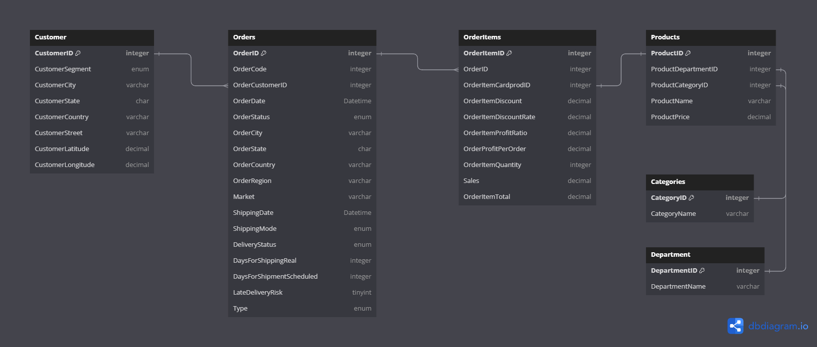
The next step involved normalizing the dataset, which essentially means organizing it in a structured way. The resulting diagram reflects the relationships and connections between different pieces of information in our dataset.

DataCo supply chain entity-relationship diagram

Normalizing tables helps eliminate redundant data, making our dataset more efficient. For example, in the department table, we now have only 11 rows with unique department names, whereas previously, these names were repeated across all 180,519 records.

With the tables now broken down and organized into its own csv file, the next step is to create a database to store these streamlined tables. This ensures that our data is well-organized and ready for efficient analysis.

I will be using MySQL and MySQL Workbench version 8.0 to perform the database creation and analysis. The following code snipe creates the tables and creates the relationship between them.

CREATE TABLE `Customers` (
  `CustomerID` integer PRIMARY KEY,
  `CustomerSegment` varchar(255),
  `CustomerCity` varchar(255),
  `CustomerState` char(2),
  `CustomerCountry` varchar(255),
  `CustomerStreet` varchar(255),
  `CustomerLatitude` decimal(8,6),
  `CustomerLongitude` decimal(9,6)
);

CREATE TABLE `Orders` (
  `OrderID` integer PRIMARY KEY,
  `OrderCode` integer,
  `OrderCustomerID` integer,
  `OrderDate` Datetime,
  `OrderStatus` varchar(255),
  `OrderCity` varchar(255),
  `OrderState` varchar(255),
  `OrderCountry` varchar(255),
  `OrderRegion` varchar(255),
  `Market` varchar(255),
  `ShippingDate` Datetime,
  `ShippingMode` varchar(255),
  `DeliveryStatus` varchar(255),
  `DaysForShippingReal` integer,
  `DaysForShipmentScheduled` integer,
  `LateDeliveryRisk` tinyint,
  `Type` varchar(255)
);

CREATE TABLE `Products` (
  `ProductID` integer PRIMARY KEY,
  `ProductDepartmentID` integer,
  `ProductCategoryID` integer,
  `ProductName` varchar(255),
  `ProductPrice` decimal(10,2)
);

CREATE TABLE `Categories` (
  `CategoryID` integer PRIMARY KEY,
  `CategoryName` varchar(255)
);

CREATE TABLE `OrderItems` (
  `OrderItemID` integer PRIMARY KEY,
  `OrderID` integer,
  `OrderItemCardprodID` integer,
  `OrderItemDiscount` decimal(10,2),
  `OrderItemDiscountRate` decimal(10,2),
  `OrderItemProfitRatio` decimal(10,2),
  `OrderProfitPerOrder` decimal(10,2),
  `OrderItemQuantity` integer,
  `Sales` decimal(10,2),
  `OrderItemTotal` decimal(10,2)
);

CREATE TABLE `Department` (
  `DepartmentID` integer PRIMARY KEY,
  `DepartmentName` varchar(255)
);

ALTER TABLE `Orders` ADD FOREIGN KEY (`OrderCustomerID`) REFERENCES `Customers` (`CustomerID`);

ALTER TABLE `Products` ADD FOREIGN KEY (`ProductDepartmentID`) REFERENCES `Department` (`DepartmentID`);

ALTER TABLE `Products` ADD FOREIGN KEY (`ProductCategoryID`) REFERENCES `Categories` (`CategoryID`);

ALTER TABLE `OrderItems` ADD FOREIGN KEY (`OrderID`) REFERENCES `Orders` (`OrderID`);

ALTER TABLE `OrderItems` ADD FOREIGN KEY (`OrderItemCardprodID`) REFERENCES `Products` (`ProductID`);

There are various ways to transfer data from Excel/csv files to a database. MySQL Workbench provides an import wizard, but due to the large number of records in the orders and orderItems files, using the wizard isn’t practical. Another option is the LOAD INFILE method, but my Workbench settings posed challenges in using this approach.

Given these constraints, I opted to develop a Python script to read each file, converting them into CSV format before generating insert SQL statements. This script ensures a more flexible and manageable way to handle the data transfer process. It’s essential to ensure that date columns are formatted correctly as YYYY-MM-DD hh:mm:ss for accurate representation in the database.

import pandas as pd
import os

def format_value(value, column_type):
    if pd.isna(value):
        return "NULL"
    elif column_type == "int64":
        return str(int(value))
    elif column_type == "float64":
        return str(float(value))
    elif column_type == "object":
        return f'"{value}"'
    else:
        return f'"{value}"'

# Read CSV file into a pandas DataFrame
csv_file_path = "file_path/csv_file_name.csv"
df = pd.read_csv(csv_file_path, encoding="utf-8")

# Specify the table name
table_name = os.path.splitext(os.path.basename(csv_file_path))[0]

# Generate SQL insert statements
sql_statements = []
for _, row in df.iterrows():
    columns = ", ".join(row.index)
    values = ", ".join(
        format_value(val, col_type) for val, col_type in zip(row.values, df.dtypes)
    )
    sql_insert = f"INSERT INTO {table_name} ({columns}) VALUES ({values});"
    sql_statements.append(sql_insert)

# Write SQL statements to a file
sql_output_file = (
    "output_file_path"
    + table_name
    + ".sql"
)  # Replace with your desired output file path
with open(sql_output_file, "w", encoding="utf-8") as f:
    f.write("\n".join(sql_statements))

print(f"SQL insert statements have been written to {sql_output_file}")

Once we’ve obtained the insert scripts for each table, the next step is to populate each table by executing the scripts in MySQL Workbench. After populating the tables, it’s crucial to perform a thorough check to ensure that all records were correctly inserted, and the relationships between tables are intact. This step helps guarantee data accuracy and integrity.

With our tables populated and verified, we’re now well-prepared for the analysis phase. This involves running SQL queries to extract insights, answer business questions, and visualize trends using tools like Tableau..

Exploratory Data Analysis

In the Customers table, we identified 20,652 unique customers, categorized into three segments: Consumer, Home Office, and Corporate. These customers are primarily located in the United States and Puerto Rico.

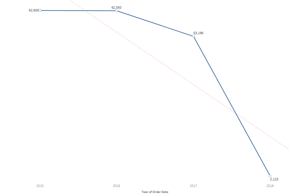
Moving on to the Orders table, we uncovered a total of 180,519 unique orders spanning from 2015 to 2018. Notably, 2018 saw the lowest order count, with 2,123 orders, as the dataset includes records only from January 2018. These orders originated from 164 countries spread across 23 regions worldwide.

Examining product prices, we found that the average price is $166.41. The price range varies from a minimum of $9.99 (Clicgear 8.0 Shoe Brush) to a maximum of $1,999.99 (SOLE E35 Elliptical). These insights lay the foundation for a deeper understanding of customer demographics, order dynamics, and product pricing within the dataset.

Analysis

What is the distribution of customers across different segments (Consumer, Corporate, Home Office)?

The distribution of customers across different segments reveals the following:

• Home Office: 3,718 customers, accounting for 18% of the total.
• Corporate: 6,239 customers, making up 30.21% of the total.
• Consumer: 10,695 customers, representing the majority at 51.79%.

What is the distribution of sales and profit per customer?

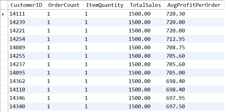
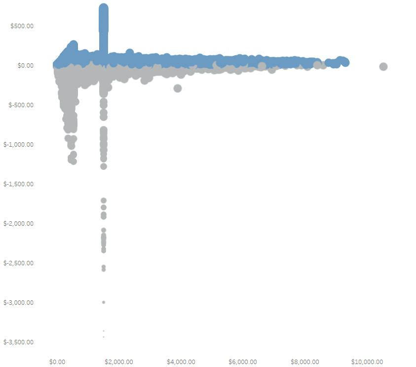
The initial impression suggests that a significant portion of the average profit per order comes from sales of products priced at $1,500, the second most expensive product. However, a closer look at customers who placed only one order unveils more nuanced findings. Among these customers:

• The maximum average profit per order is $720.30.
• The minimum average profit per order is -$3,442.50, indicating a loss.
• There are 1,584 orders that resulted in a loss.

These insights shed light on the variability in profitability across different products and customer behaviors. Understanding both the highs and lows in average profit per order is crucial for making informed business decisions.

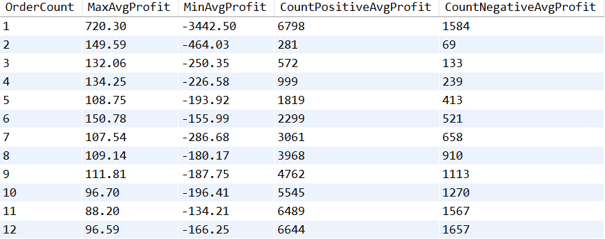
Let’s analyze how this numbers change across different group of orders count.

The above image illustrates a subset of the maximum and minimum average profit for customers who placed one order, two orders, and so forth. It also includes the count of orders that produced positive and negative profits. From this analysis, we can draw several inferences:

• Customers who placed a single order tend to generate the majority of negative profits.
• Overall, 80.63% of the orders result in positive profits.
• About 18.71% of the total orders yield negative profits.
• A minor portion, 0.65% of orders, did not generate any profits.

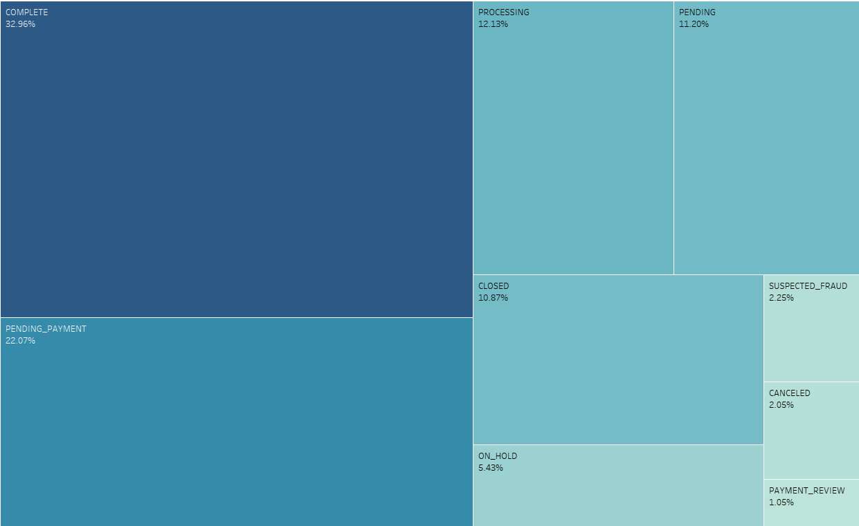
What is the distribution of order statuses?

Although 2.25% of all orders has a status of SUSPECTED_FRAUD, it is worth take a look into this

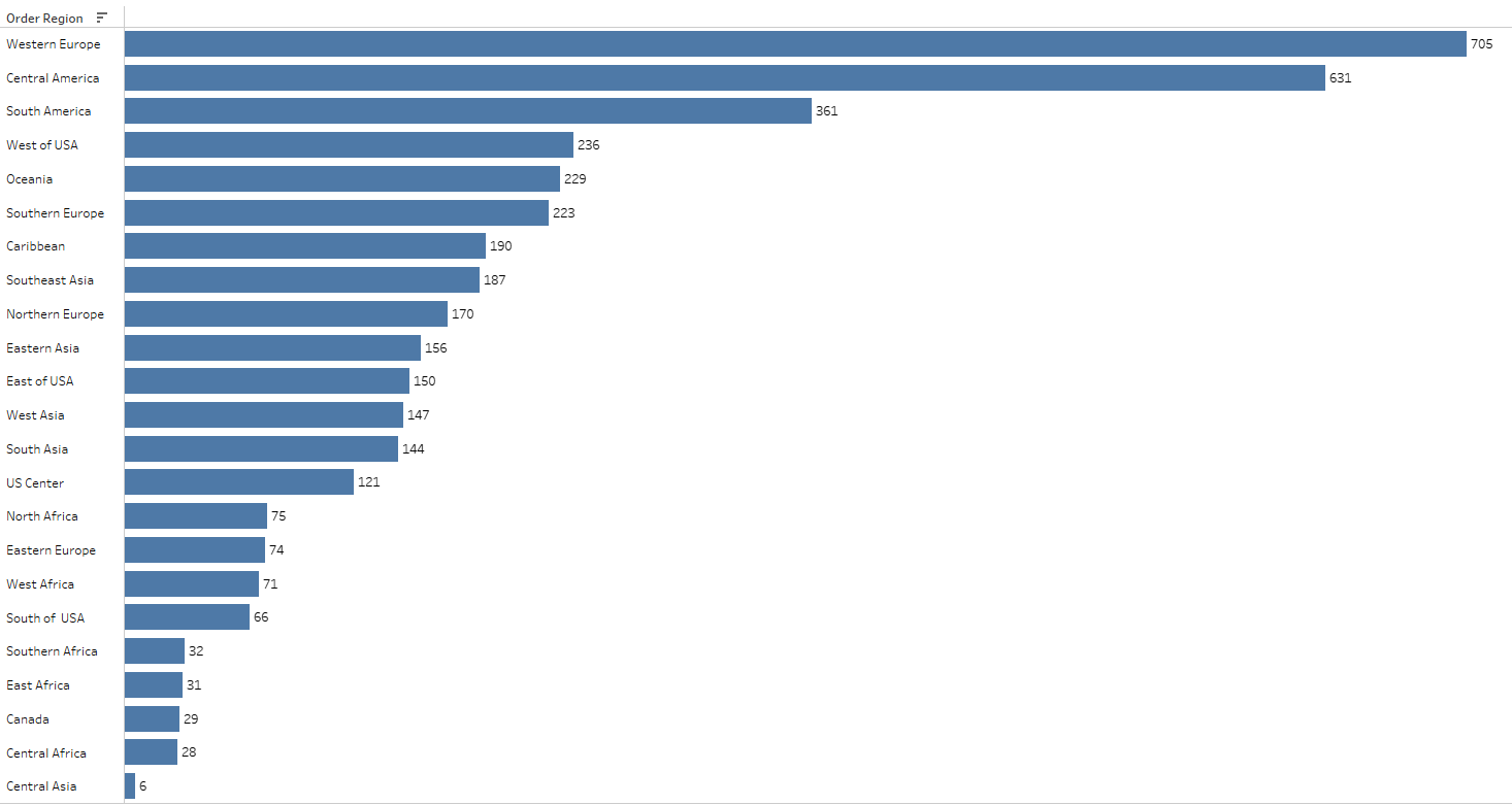
The analysis reveals interesting patterns in orders flagged with a SUSPECTED_FRAUD status across different regions. Notably, Western Europe and Central America show the highest count of orders with SUSPECTED_FRAUD status, while Central Asia has the lowest.

Exploring further, there are 1,429 unique customers associated with this suspected fraud status. A specific query was crafted to identify customers solely engaged in transactions marked as SUSPECTED_FRAUD. The query results in 202 customers who have placed one or more orders, all of which are flagged as suspected fraud. It’s noteworthy that these transactions exclusively involve the payment type TRANSFER.

This insight prompts considerations about the nature of these transactions and raises the possibility that these customers may have attempted fraudulent activities, given the absence of diverse order statuses in their transaction history.

How is the on-time delivery performance?

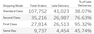
55% of all orders result in late deliveries. The average late delivery day is 1.62 days, the minimum days late of a order is 1 day and the maximum days of late deliveries is 4 days. Central America (15.68%), Western Europe (15.30%) and South America (8.19%) has the highest late delivery percentage.

Given the absence of explicit information regarding customer-paid delivery fees in the dataset, an assumption has been made for the analysis. It is presumed that customers incur different fees based on the selected shipping mode, with the hierarchy being Same Day > First Class > Second Class > Standard Class.

Under this assumption, the analysis indicates potential areas for improvement, specifically concerning the percentage of late deliveries for first-class and same-day shipments. This observation underscores the importance of studying factors that influence the timeliness of orders, offering valuable insights for stakeholders seeking to optimize delivery performance.

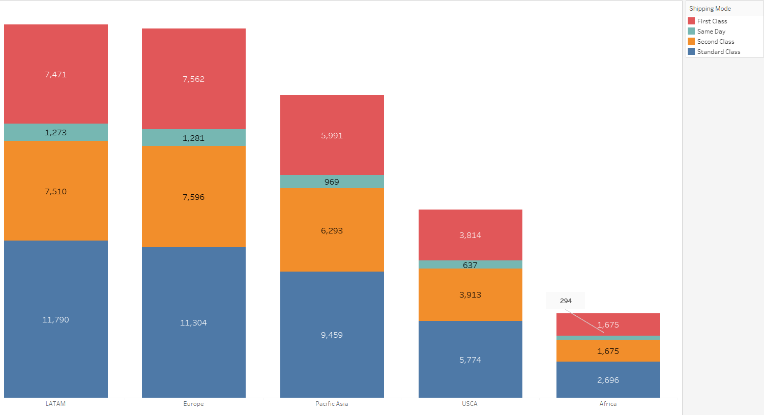
How does the choice of shipping mode vary across different markets?

Based on the above table there is not a big difference across markets with respect shipping mode. Orders that come from LATAM tend to have the majority of standard class mode followed by Europe.

Analyze the distribution of orders over time (daily, monthly, yearly).

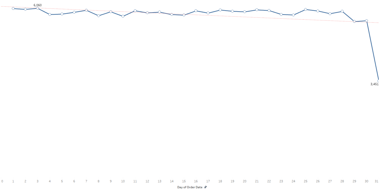
Understanding the order date range, which spans from January 2015 to January 2018, provides context for the distribution analysis. On a daily basis, the dataset shows an average of 5,823 orders. Notably, the day with the highest order count is the third day, recording 6,060 orders, while the 31st day sees the lowest at 3,451 orders. Across days, there is observable fluctuation, but the majority surpass the daily average.

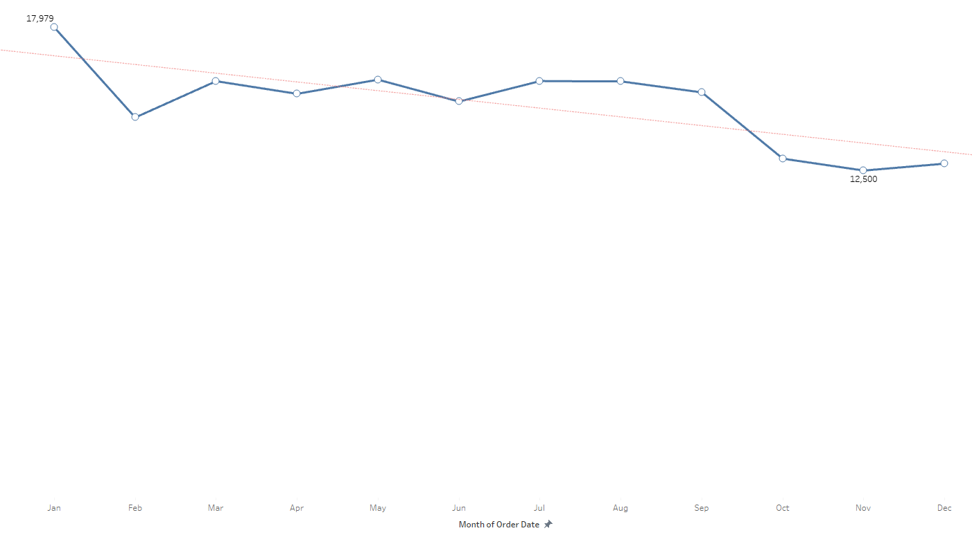
Moving to the monthly distribution, the average stands at 15,043 orders. January emerges as the month with the highest orders, influenced by the exclusive data from January 2018. February, October, November, and December fall below the monthly average, with November recording the lowest at 12,500 orders.

Yearly distribution indicates relatively stable figures, except for 2018, which appears as the lowest due to the dataset’s limited orders from January of that year.

Identify any seasonality patterns in sales or order volume.

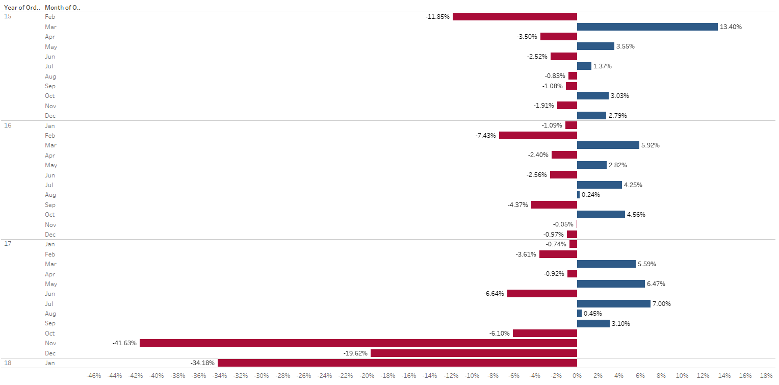
There are fluctuations in monthly sales throughout the years, indicated by positive and negative percentage changes. This suggests varying patterns in consumer behavior or market conditions. Certain months consistently show positive or negative trends across multiple years. For instance, November and December of 2017 exhibit significant negative changes, possibly influenced by holiday-related factors. Examining the yearly changes, there’s a notable drop in January 2018 (-34.18%). Due to the limited dataset for that month or specific market conditions during that period. Months like November 2017 and January 2018 experienced substantial negative changes, indicating potential challenges or external factors affecting sales during those specific periods. Some months, such as March 2015 and June 2017, demonstrate relative stability with smaller percentage changes, suggesting consistent sales patterns.

---

Project Recommendations:

1. Fraud Prevention:

• Objective: Enhance security measures to prevent fraudulent activities.
• Action Steps:
  • Investigate customers involved in suspected fraud with a focus on those with TRANSFER payment types.
  • Collaborate with the security team to implement additional safeguards for such transactions.
• Expected Impact: Minimize the occurrence of fraudulent activities, improving overall transaction security.

2. Delivery Optimization:

• Objective: Improve on-time delivery performance, especially for first-class and same-day deliveries.
• Action Steps:
  • Analyze factors contributing to late deliveries and address operational inefficiencies.
  • Implement corrective actions based on identified challenges in the delivery process.
• Expected Impact: Enhance customer satisfaction and loyalty by ensuring timely order deliveries.

3. Sales Strategies:

• Objective: Optimize sales and pricing strategies for improved profitability.
• Action Steps:
  • Leverage insights from sales and profit analysis to refine marketing campaigns.
  • Explore factors influencing positive and negative profit outcomes for strategic adjustments.
• Expected Impact: Increase sales revenue and profitability through targeted marketing and pricing.

Tableau Dashboard

Tableau Public DataCo Dashboard